Poster: The Strength and Bound of Temporal Correations
More details on the work in the following poster (and more!) can be found at arXiv:1510.04425 and at J. Phys. A: Math. Theor. 50, 055302 (2017).
This poster was presented at CQD2015.
The Strength and Bound of Temporal Correations
1School of Physics & Astronomy, Monash University, Victoria 3800, Australia
2School of Physical and Mathematical Sciences, Nanyang Technological University, Singapore and Centre for Quantum Technologies, National University of Singapore, Singapore
3School of Mathematics and Physics, Queens University, Belfast BT7 1NN, United Kingdom
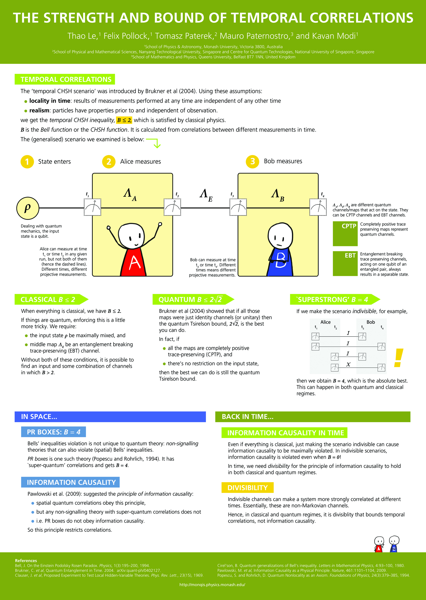
Temporal Correlations
The 'temporal CHSH scenario' was introduced by Brukner et al (2004). Using these assumptions:
- locality in time: results of measurements performed at any time are independent of any other time
- realism: particles have properties prior to and independent of observation.
we get the
\(B\) is the
The (generalised) scenario we examined is below:
(Main Figure)
The main figure consists of a two boxes representing two different laboratories. In each box is a picture of a person: Alice on the left and Bob on the right. Alice has their arms in the air, and Bob's arms are folded across their front. A circle representing the quantum state crosses through the two boxes. Where its path meets a line of the box, there is a measurement box with a dotted outline. The system state \( \rho\) first crosses Alice's box at time \(t_1\), then passes through the CPTP map \( \Lambda_A \); it exits Alice's laboratory at time \( t_2 \), passes through the CPTP map \( \Lambda_E \), then enters Bob's laboratory at time \( t_3 \), passes through CPTP map \( \Lambda_B \) and finally exits Bob's laboratory at time \( t_4 \).
- State enters
- Alice measures
- Bob measures
The notes on the figure are:
- Dealing with quantum mechanics, the input state is a qubit.
- Alice can measure at time \( t_1\) or time \( t_2\) in any given run, but not both of them (hence the dashed lines). Different times, different projective measurements.
- Bob can measure at time \(t_3\) or time \(t_4\). Different times means different projective measurements.
- \(\Lambda_A\), \(\Lambda_E\), \(\Lambda_B\) are different quantum channels/maps that act on the state. They can be CPTP channels and EBT channels.
- CPTP Completely positive trace preserving maps represent quantum channels.
- EBT Entanglement breaking trace preserving channels, acting on one qubit of an entangled pair, always results in a separable state.
Classical \(B \leq 2\)
When everything is classical, we have \(B\leq2\). If things are quantum, enforcing this is a little more tricky. We require:
- the input state \(\rho\) be maximally mixed, and
- middle map \(\Lambda_E\) be an entanglement breaking trace-preserving (EBT) channel.
Without both of these conditions, it is possible to find an input and some combination of channels in which \(B>2\).
Quantum \(B \leq 2 \sqrt{2} \)
Brukner et al (2004) showed that if all those maps were just identity channels (or unitary) then the quantum Tsirelson bound \( 2\sqrt{2}\) is the best you can do.
In fact, if
- all the maps are completely positive trace-preserving (CPTP), and
- there's no restriction on the input state,
then the best we can do is still the quantum Tsirelson bound.
'Superstrong' \(B = 4\)
If we make the scenario
A figure is displayed, showing all the combinations of measurements Alice and Bob can make: there is an identity channel between the combinations of measurements times \( (t_1, t_3) \), \( (t_1, t_4) \), and \( (t_2, t_3) \). However, there is a bit flip X channel in-between measurement times \( (t_2, t_4) \). A large yellow exclaimation mark draws attention to this.
then we obtain \(B=4\), which is the absolute best. This can happen in both quantum and classical regimes.
In space...
PR Boxes: \(B=4\)
Bells' inequalities violation is not unique to quantum theory:
Information Causality
Pawlowski et al. (2009): suggested the
- spatial quantum correlations obey this principle,
- but any non-signalling theory with super-quantum correlations does not
- i.e. PR boxes do not obey information causality.
So this principle restricts correlations.
Back in time...
Information causality in time
Even if everything is classical, just making the scenario indivisible can cause information causality to be maximally violated. In indivisible scenarios, information causality is violated even when \(B=0\)!
In time, we need
Divisibility
Indivisible channels make a system more strongly correlated at different times. Essentially, these are non-Markovian channels.
Hence, in classical and quantum regimes, it is divisiblity that bounds temporal correlations, not information causality.
References
- Bell, J. On the Einstein Podolsky Rosen Paradox.
Physics , 1(3):195-200, 1994. - Brukner, C.
et al , Quantum Entanglement in Time. 2004. arXiv:quant-ph/0402127 - Clauser, J.
et al , Proposed Experiment to Test Local Hidden-Variable Theores.Phys. Rev. Lett. , 23(15), 1969. - Cirel'son, B. Quantum generalizations of Bell's inequality.
Letters in Mathematical Physics , 4:93-100, 1980. - Pawlowski, M.
et al , Information Causality as a Physical Principle.Nature , 461:1101-1104, 2009. - Popescu, S. and Rohrlich, D. Quantum Nonlocality as an Axiom.
Foundations of Physics , 24(3):379-385, 1994.